Nerual Networks

1 Nerual Networks

Recall that in the housing price prediction example. We take the size of the house as input and make predictions on price by fitting a straight line. The problem in this model is that a straight line has mathematical meaning in negative domain, which does not make sense in predicting house values. Thus, we need to perform some link function to get a plot like the one below.

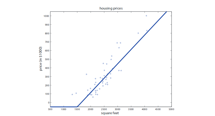
Mathematically, we want $f:x\rightarrow y$. To prevent a negative prediction, we can have a single neuron where $f(x) = \max(ax+b,0)$ for some a and b from training process. This is called ReLU (rectified linear unit) function. This is essentially the simplest neuron that we can have. We can also stack multiple neurons where the output of a neuron can serve as the input of the other. This can give us a more complex struture.

In the housing price prediction example, we can have multiple input such as the size of house, the number of bedrooms, the zip code and the wealth of neighborhood. We can take these features as input to the neural network. In addition, we might also find out that the size of house and the number of bedrooms are related to family size, the zip code is related to the walkable distance to stores and the wealth of neighborhoods are related to the quality of life around. Thus, we can futher say that the price of house depends more directly on these three factors. Such an idea can be realized by stacking several neurons together as:

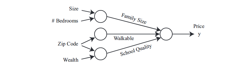
Part of magic of neural networks is that we only need to feed the network with input features x and output prediction y. Everything else is called hidden units and figured out by the neural network itself. They are called hidden layers since we do not have ground truth for those nuerons and we ask network to solve for us. We cal this end-to-end learning. The last thing required is a large amount of training samples. The model will figure out the latent features that are helpful on prediction. Since human cannot understand the features it has produced, this renders the neural network as black box technology.

Before going to details, let’s denote $x_i$ as i-th input feature, $a_j^{[\ell]}$ as the activition output at j-th unit in layer $\ell$, $foo^{\ell}$ as everything associated with layer $\ell$ and $z=\theta^Tx$. We can draw a diagram for a single neuron for illustration as:

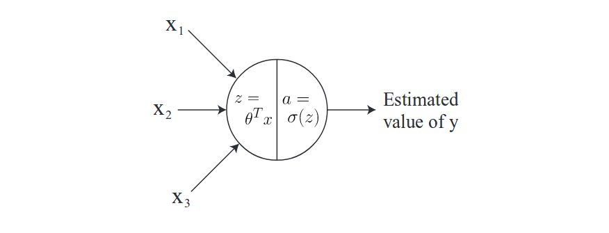
For the choice of activition functions, we can logistic function as before:

\[g(x) = \frac{1}{1 + \exp(-w^Tx)}\]

In addition, we can have more:

\[g(z) = \frac{1}{1+\exp(-z)}\quad\text{sigmoid}\] \[g(z) = \max(z,0)\quad\text{ReLU}\] \[g(z) = \frac{\exp(z) - \exp(-z)}{\exp(z) + \exp(-z)}\quad\text{tanh}\]

Back to neuron network of price prediction, what it does for first hidden unit at first hidden layer is:

\[z_1^{[1]} = W_1^{[1]}x + b_1^{[1]} \quad \text{and} \quad a_1^{[1]} = g(z_1^{[1]})\]

where W is parameter matrix and $W_1$ is first row of it and b is a scalar. Similarly, we can have:

\[z_2^{[1]} = W_2^{[1]}x + b_2^{[1]} \quad \text{and} \quad a_2^{[1]} = g(z_3^{[1]})\] \[z_3^{[1]} = W_3^{[1]}x + b_3^{[1]} \quad \text{and} \quad a_3^{[1]} = g(z_3^{[1]})\]

So the output of first layer from activition function can be defined as:

\[a^{[1]} = \begin{bmatrix} a_1^{[1]}\\ a_2^{[1]} \\ a_3^{[1]} \\ a_4^{[1]} \end{bmatrix}\]

For some of tasks, we might not want to use ReLU although it is really popular in research simply becuase it is not always correct that we should have non-negative value for prediction.

2 Vectorization

Now, a natural question to ask is that what the activation does and what if I remove it. Intuitively, activition functions are the key part of making deep learning work and making it possible to model non-linear relationships. Without it, what neural network does simply becomes linear combinations between weights and its input. Let’s see how mathematically we can prove this.

In the previous section, we calculate each $z_i^{[1]}$ and apply activation function for each of them. We can put all of them into a matrix and take advantage of matrix calculations to speed up this process.

2.1 Vectorizaing the Output Computation

So for the first layer, we can have:

\[\underbrace{\begin{bmatrix} z_1^{[1]}\\ z_2^{[1]} \\ z_3^{[1]} \\ z_4^{[1]} \end{bmatrix}}_{z^{[1]}\in\mathcal{R}^{4\times 1}} = \underbrace{\begin{bmatrix} -(W_1^{[1]})^T-\\ -(W_2^{[1]})^T- \\ -(W_3^{[1]})^T- \\ -(W_4^{[1]})^T- \end{bmatrix}}_{W^{[1]}\in\mathcal{R}^{4\times 3}}\underbrace{\begin{bmatrix} x_!\\ x_2 \\ x_3 \end{bmatrix}}_{x\in\mathcal{R}^{3\times 1}} + \underbrace{\begin{bmatrix} b_1^{[1]}\\ b_2^{[1]} \\ b_3^{[1]} \\ b_4^{[1]} \end{bmatrix}}_{b^{[1]}\in \mathcal{R}^{4\times 1}}\]

The dimenion of each matrix is labelled below. In short, it is $z^{[1]} = W^{[1]}x + b^{[1]}$, which is linear relationship. Then, we can apply activition function on z vector like sigmoid function for example. Similarly, we can use matrix to represent the propagation from first layer to secon layer. As you can see here, without non-linear activition function, we simply do linear regression here, which cannot model many complicated non-linear relationship.

2.2 Vectorization over Training Examples

Now, we want to do this thing for all the training samples that going to be fed into neural network. We want to do it at one time. So we define a sample matrix:

\[X = \begin{bmatrix} \lvert & \lvert & \lvert\\ x^{(1)} & x^{(2)} & x^{(3)} \\ \lvert & \lvert & \lvert \end{bmatrix}\]

So we can get the outpout as :

\[Z^{[1]} = \begin{bmatrix} \lvert & \lvert & \lvert\\ z^{[1](1)} & z^{[1](2)} & z^{[1](3)} \\ \lvert & \lvert & \lvert \end{bmatrix} = W^{[1]}X + b^{[1]}\]

Meanwhile, we also (as always) need to define the objective function that we want to maximize. For binary class, we can have the objective function as :

\[\sum\limits_{i=1}^m \big( y^{(i)}\log a^{[2] (i)} + (1 - y^{(i)})\log (1 - a^{[2] (i)})\big)\]

where $a^{[2] (i)}$ is the output from second layer (also the final layer) for i-th training sample. Remember that we are trying to model a binary problem, which is usually a Bernoulli. Thus, the output from neural network should be in class 1 with probability $a^{[2] (i)}$. We take log for this Bernoulli and you will get the above with math manipulation.

We can use gradient ascent for updating.

3 Backpropagation

We have defined and learned how neural network propagates forwards, which is called prediction stage. Now, we want to know how neural network propagates backwards, which is called learning stage.

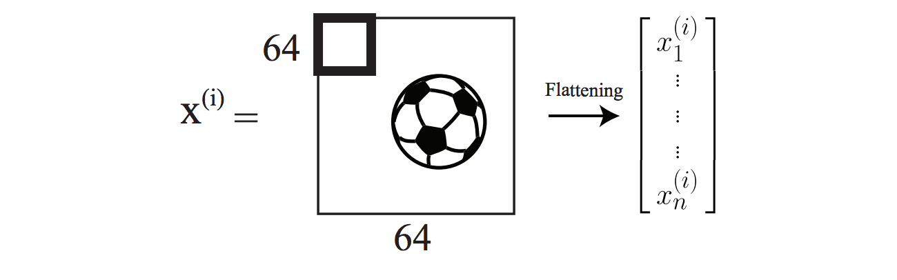
For example, assume that we want to predict if an image contains a ball or not, which is a binary problem. As an image, we have RGB values, which means we deal with a three dimensional matrix. We first flatten it to a one-dimensional vector, and then feed it into the neural network to get the output. It can be illustrated figuratively as below.

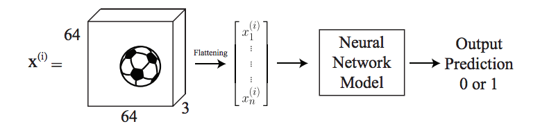
So next, let’s talk about how to update its parameters.

3.1 Parameter Initialization

Keep in mind that the input is flattened although it is image. With two layers of neural network, we can draw it as:

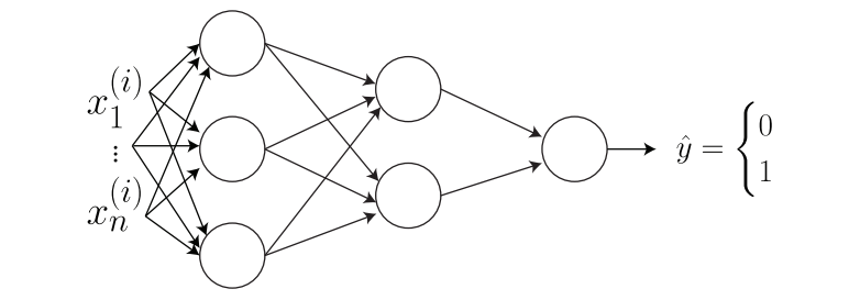
Note how each node in each layer is connected. This is called fully connected. We can now use the method discussed in last section to figure out what output will be for each node in each layer by using matrix notation. In addition, with matrix notation, we can calculate the number of parameters that we are trying to update. I would not repeat the calculation step but the answer is $3n+14$.

Before updating, we need to initialize these parameters. We CANNOT initialize them to zero since this will cause the output of first layer to be zero and further problem when we update them (gradient will be same). The workaround is to initialize them by unit Gaussian.

After initialization and one single input, we then have the prediction $\hat{y}$. We can use this value to back-propagate so that network can learn from it. If $\hat{y} = y$, then we have nothing to learn. The network does well. However, if not, we have something to ask for network to update its parameters so that it can do better next time. Is it like a human, isn’t?

Let’s define the loss function as :

\[\mathcal{L}(\hat{y},y) = -\Big[(1-y)\log (1 - \hat{y}) + y\log (\hat{y})\Big]\]

The loss function can basically tell the network about what we really care about. So the network knows what the evaluation scheme is during the training.

Given a layer index $\ell$, we can update them:

\[W^{[\ell]} = W^{[\ell]} - \alpha\frac{\partial \mathcal{L}}{\partial W^{[\ell]}}\] \[b^{[\ell]} = b^{[\ell]} - \alpha\frac{\partial \mathcal{L}}{\partial b^{[\ell]}}\]

where $\alpha$ is the learning rate.

There are two cases that I want to discuss.

(1) What will happen if we initialize all the parameters to zeros? In this case, we can plug it back to matrix calculation, which will be zero as output. This is also the input to sigmoid function, leading to 0.5 ALWAYS.

(2) What will happen if we initialize all the parameters to the same values? In this case, from matrix calculation, we can see that this can cause that output from each node in that layer will have all the same values. This will occur to each layer. When we calculate the gradient, this will give us the same gradient in each node in a layer. It will learn the same thing for each neuron.

Instead, we have something better than Gaussian, called Xavier/He initialization. We initialize it as:

\[w^{[\ell]} \sim \mathcal{N}(0,\sqrt{\frac{2}{n^{[\ell]} + n^{[\ell-1]}}})\]

where $n^{[\ell]}$ is the number of neurons in layer $\ell$.

3.2 Optimization

In the simple neural network above, we have several parameters to update, namely $W^{[1]},b^{[1]},W^{[2]},b^{[2]},W^{[3]},b^{[3]}$. We can use stochastic gradident descent to optimize. That is, we find the derivative with respect to each variable and take a step of it. Let’s look at $W^{[3]}$.

\[\begin{align} \frac{\partial \mathcal{L}}{\partial W^{[3]}} &= -\frac{\partial}{\partial W^{[3]}}\frac{\partial \mathcal{L}}{\partial W^{[3]}}\frac{\partial \mathcal{L}}{\partial W^{[3]}}\bigg((1-y)\log(1-\hat{y}) + y\log\hat{y}\bigg)\\ &= -(1-y)\frac{\partial}{\partial W^{[3]}}\log\bigg(1-g(W^{[3]}a^{[2]}+b^{[3]})\bigg) \\ & - y\frac{\partial}{\partial W^{[3]}}\log\bigg(g(W^{[3]}a^{[2]}+b^{[3]})\bigg) \\ &= -(1-y)\frac{1}{1-g(W^{[3]}a^{[2]}+b^{[3]})}(-1)g^{\prime}(W^{[3]}a^{[2]}+b^{[3]})a^{[2] T}\\ & -y\frac{1}{1-g(W^{[3]}a^{[2]}+b^{[3]})}g^{\prime}(W^{[3]}a^{[2]}+b^{[3]})a^{[2] T}\\ & = (a^{[3]}-y)a^{[2] T} \end{align}\]

where g is sigmoid function.

In order to compute the gradient for $W^{[2]}$, we have to use chain rule from calculus, which will give us as:

\[\frac{\partial \mathcal{L}}{\partial W^{[2]}} = \frac{\partial \mathcal{L}}{\partial a^{[3]}}\frac{\partial a^{[3]}}{\partial z^{[3]}}\frac{\partial z^{[3]}}{\partial a^{[2]}}\frac{\partial a^{[2]}}{\partial z^{[2]}}\frac{\partial z^{[2]}}{\partial W^{[2]}}\]

Note that each fraction shows the dependence between numerator and denominator.

Now, we can plug in each one:

\[\frac{\partial \mathcal{L}}{\partial W^{[2]}} = \underbrace{\frac{\partial \mathcal{L}}{\partial a^{[3]}}\frac{\partial a^{[3]}}{\partial z^{[3]}}}_{a^{[3]} - y}\underbrace{\frac{\partial z^{[3]}}{\partial a^{[2]}}}_{W^{[3]}}\underbrace{\frac{\partial a^{[2]}}{\partial z^{[2]}}}_{g^{\prime}(z^{[2]})}\underbrace{\frac{\partial z^{[2]}}{\partial W^{[2]}}}_{a^{[1]}}\]

Traditionally, we need to use generalized Jacobian matrix for this calculation. If you are not familiar with this, you can check my post on math. However, we won’t do this here since generalized Jacobian matrix calculation will require a lot of memory. We have to work around it.

I do suggest to take a look at this post and this post for detailed explanation. Here, I just keep it simple to get:

\[\frac{\partial \mathcal{L}}{\partial W^{[2]}} = \underbrace{(a^{[3]}- y)}_{1\times 1}\underbrace{W^{[3]^T}}_{2\times 1}\odot\underbrace{g^{\prime}(z^{[2]})}_{2\times 1}\underbrace{a^{[1]}}_{1\times 3}\]

where $\odot$ denotes element-wise product. What happens here, in short, is that the first term is scalar but $W^{[3]^T}\odot g^{\prime}(z^{[2]})$ this part is originally a generalized Jacobian matrix multiplication. However, since the activition function is per element, the generalized Jacobian matrix for $\frac{\partial a^{[2]}}{\partial z^{[2]}}$ is a 2 by 2 diagnoal matrix. And $\frac{\partial z^{[3]}}{\partial a^{[2]}}$ is actually a 1 by 2 vector. The matrix multiplication of the two can be calculated in another way which is element-wise product. Looking back to the architecture of the nerual network, we can see that the gradient of $W^{[3]}$ is back-propegated seperately to layer 2. So intuitively, the gradient should only affect them individually. That’s why we use element-wise product and the dimensions seems “wrong”.

For the last term, the reason that it is not a generalized Jacobian is that we can work around it by just getting the matrix as a result. More details can be found the linked posts above.

Now, we can use the gradient descent for updating:

\[W^{[\ell]} = W^{[\ell]} - \alpha\frac{J}{W^{[\ell]}}\]

where J is the cost function defined as $J=\frac{1}{m}\sum\limits_{i=1}^m\mathcal{L}^i$.

Another popular optimization algorithm is called momentum. The update rule is:

\[\begin{cases} v_{dW^{[\ell]}} = \beta dW^{[\ell]} + (1-\beta)\frac{\partial J}{dW^{[\ell]}} \\ W^{[\ell]} = W^{[\ell]} - \alpha v_{dW^{[\ell]}}\\ \end{cases}\]

This rule happens in two stages. The first one is to get the speed and the second is to use the speed to update it. This algorithm basically keeps track of all the past gradient and will help escape from saddle point.

3.3 Analyzing the Parameters

We have done all the components in the training process. If we have trained model which performs 94% on training dataset but only 60% in testing dataset, then there is an overfitting. The possible solutions are: collecting more data, employing regularization or making the model simpler/shallower. In this section, I am going to talk about regularization.

L2 Regularization

Let W donote all the parameters in the model. The L2 regularization adds another term to the cost function, which is called reluarizer:

\[\begin{align} J_{new} &= J_{old} + \frac{\lambda}{2}\lvert\lvert W \rvert\rvert^2 \\ &=J_{old} + \frac{\lambda}{2}\sum\limits_{i,j}\lvert W_{ij}\rvert^2\\ &=J_{old} + \frac{\lambda}{2}W^TW \end{align}\]

where $\lambda$ is an arbitrary value. If it is large, it means a parge penalty and large regularization. Then, the update rule has also changed to:

\[\begin{align} W &= W - \alpha\frac{\partial J}{\partial W} - \alpha\frac{\lambda}{2}\frac{\partial W^TW}{\partial W}\\ &= (1-\alpha\lambda)W - \alpha\frac{\partial J}{\partial W} \end{align}\]

This means that in updating, some penalties might be included in order to optimize the new J overall. Note that this penalty encourages parameters to be small in L2 magnitude. This is becuase larger magnitude of parameters results in larger varaince.

Parameter Sharing

Recall that logistic regression train each parameter for each pixel. However, for ball detection task, if the ball always appears in the center pixels in the training dataset, this might be a problem if a ball appears in a cornor in testing phase. This is because the wieghts on the cornor have never been trained with a ball in there so that the weights do not have that concepts in them.

To solve this, we have a new type of network structure called comvolutional neural networks. Instead of a vector of parameters, we use a matrix of vector, say size of 4 by 4. We take this matrix and slide it over the image. This can be shown below.

This matrix of parameters will take inner product with corresponding pixels in the image, which is a scalar. Then we slide matrix to the right and the bottom, which can be shown as:

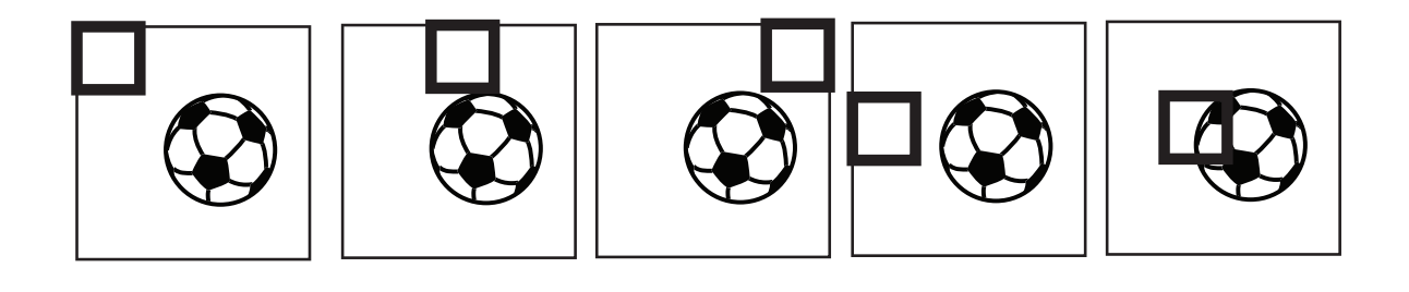
Note that each matrix share the same weighs across the entire image.