Discriminative Algorithm
A Chinese version of this section is available. It can be found here. The Chinese version will be synced periodically with English version. If the page is not working, you can check out a back-up link here.
A classical learning paradigm is called supervised learning. In this case, we usually have an input called features and output called target. The goal is that given some features we ask the trained model to predict the output.
To do so, we collect a training dataset in which we have a number of pairs of training sample composing of a feature vector denoted $\mathcal{X}$ and its corresponding output denoted $\mathcal{Y}$. Since we have ground truth for every single input, we call this type of learning as supervised learning and the learned model as hypothesis. An example can be shown in the table below.
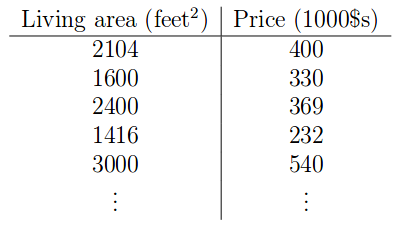
In this case, we have living areas as features and price as output. The task is that given a new input of living area, the model can predict the price of it.
When the target output is in continuous space, we call it a regression problem. When the target output is in discrete space, we call it as a classification problem.
1 Linear Regression
A linear regression probelm can be models as :
\[h(x) = \sum\limits_{i=0}^n \theta_i x_i = \theta^Tx\]We have $\theta_0$ for the bias and sometimes it is called intercept term. Imagine that you try to regress for a line in 2D domain, the intercept term basically determines where the line crossed y-axis. $\theta$ is called parameters which we want to learn from training data.
To learn it, we also define the cost function on which we are trying to minimize:
\[J(\theta) = \frac{1}{2}\sum\limits_{i=1}^m (h_{\theta}(x^{(i)}) - y^{(i)})^2\]The goal is to find such $\theta$ that minimize the cost. The question is how. You might want to know why there is $\frac{1}{2}$. It will be clear when we derive the derivative of this cost function in the following section. In short, it is mathematically convenient to define that way.
Least Mean Sqaure(LMS) algorithm
LMS algorithm essentially uses gradient descent to find the local min. To implement it, we start an initial guess $\theta = \overrightarrow{0}$ and then update repeatedly as:
\[\theta_j = \theta_j - \alpha \frac{\partial}{\partial \theta_j}J(\theta)\]where j spans all the components in feature vector. $\alpha$ is called learning rate,controlling how fast it learns.
Now,we can solve the partial derivative with respect to one sample as :
\[\begin{align} \frac{\partial}{\partial \theta_j}J(\theta) &= \frac{\partial}{\partial \theta_j} \frac{1}{2} (h_{\theta}(x)-y)^2\\ &= 2\frac{1}{2}(h_{\theta}(x)-y) \frac{\partial}{\partial \theta_j} (h_{\theta}(x)-y)\\ &= (h_{\theta}(x)-y) \frac{\partial}{\partial \theta_j}(\sum\limits_{i=0}^n \theta_i x_i - y) \\ &= (h_{\theta}(x)-y) x_j \end{align}\]Math: The second line is rsulted from chain rule of derivatives. On third line, I expand $h_{\theta}(x) = \sum\limits_{i=0}^n \theta_i x_i$ by definition. On last line, since we only care about $\theta_j$, everything else is constant.
So the update for all the samples are:
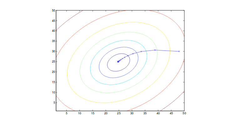
\[\theta_j = \theta_j + \alpha\sum\limits_{i=0}^m (y^{(i)} - h_{\theta}(x^{(i)}))x_j^{(i)}\]where m is the number of training samples and j can span the dimension of feature vector. This algorithm takes all the factors from every single training sample. We call it batch gradient descent. This method is sensitive to the local minimum (i.e. might arrive at saddle point) where we generally assume that the cost function has only global minimum which is the case (J is convex). An graphical illustration can be shown below.
Note that in the updating, we run through all the samples to make one step forward to local min. This step is computationally expensive if m is very large. Thus,in this case, we introduce a similar algortihm called stochastic gradient descent where only a small part of samples are fed into the algorithm at one time. By doing this, we can converge faster although it might oscillate a lot. It will produce good approximation to the global minimum. Thus, we use this often in reality.
2 Normal Equations
In the section above, we use the iterative algorithm to find the minimum. This method is used usually when the solution of the derivative w.r.t. parameters equal to zero is intractable (i.e. cannot be solved easily). If we are able to find the derivative and solve when it is zero, we can explicitly calculate the local minimum. Before going through, we need the memory refresher for the math!
Matrix derivatives
Some of the concepts are discussed in the other post,which you can find it here.
In this subsection, I will talk about trace operator in linear algebra. Basically, the trace operation is defined as:
\[trA = \sum\limits_{i=1}^n A_{ii}\]where A must be a square matrix. Now, I will list the properties of trace and write proof if time permitted.
\[trAB = trBA\]Proof:
\[\begin{align} trAB &= \sum\limits_{i=1}^N (AB)_{ii} \\ &= \sum\limits_{i=1}^N \sum\limits_{j=1}^M A_{ij}B_{ji} \\ &= \sum\limits_{j=1}^M \sum\limits_{i=1}^N B_{ji} A_{ij}\\ &= trBA \blacksquare \end{align}\] \[trABC = trCAB = trBCA\]Proof:
\[\begin{align} trABC &= \sum\limits_{i=1}^N (ABC)_{ii} \\ &= \sum\limits_{i=1}^N \sum\limits_{j=1}^M \sum\limits_{p=1}^K A_{ij}B_{jk}C_{ki} \\ &= \sum\limits_{p=1}^K \sum\limits_{i=1}^N \sum\limits_{j=1}^M C_{ki}A_{ij}B_{jk}\\ &= trCAB \blacksquare \end{align}\]The other is similar the proof above. Note that you cannot randomly shuffle the order of each matrix because of the dimensionality constraint.
\[trABCD = trDABC = trCDAB = trBCDA\]Proof: Similar to the above.
\[trA = trA^T\]Proof:
\[\begin{align} trA &= \sum\limits_{i=1}^N A_{ii} \\ &= \sum\limits_{i=1}^N A_{ii}^T \\ &= trA^T \blacksquare \end{align}\] \[tr(A+B) = trA + trB\]Proof:
Similar to the above.
\[tr\alpha A = \alpha trA\]Proof:
Similar to the above.
\[\triangledown_A trAB = B^T\]Proof:
\[\begin{align} \triangledown_{A_ij} trAB &= \sum\limits_{i=1}^N (AB)_{ii} \\ &= \sum\limits_{i=1}^N \sum\limits_{j=1}^M A_{ij} B_{ji} \\ &= B_{ji} \end{align}\]We know that:
\[\triangledown_A trAB = \begin{bmatrix} \frac{\partial trAB}{\partial A_{11}} & \frac{\partial trAB}{\partial A_{12}} & \dots & \frac{\partial trAB}{\partial A_{1M} }\\ \frac{\partial trAB}{\partial A_{21} } & \frac{\partial trAB}{\partial A_{22} } & \dots & \frac{\partial trAB}{\partial A_{2M} } \\ \vdots & \vdots & \dots & \vdots \\ \frac{\partial trAB}{\partial A_{N1} } & \frac{\partial trAB}{\partial A_{N2} } & \dots & \frac{\partial trAB}{\partial A_{NM}} \end{bmatrix}\]Plug it in, we found out:
\[\triangledown_A trAB = B^T\] \[\triangledown_{A^T}f(A) = (\triangledown_A f(A))^T\]Proof:
Assume $f:\mathbb{R}^{M\times N}\rightarrow\mathbb{R}$, we have:
\[\begin{align} \triangledown_{A^T} f(A) &= \begin{bmatrix} \frac{\partial f}{\partial (A^T)_{11}} & \frac{\partial f}{\partial (A^T)_{12}} & \dots & \frac{\partial f}{\partial (A^T)_{1M} }\\ \frac{\partial f}{\partial (A^T)_{21} } & \frac{\partial f}{\partial (A^T)_{22} } & \dots & \frac{\partial f}{\partial (A^T)_{2M} } \\ \vdots & \vdots & \dots & \vdots \\ \frac{\partial f}{\partial (A^T)_{N1} } & \frac{\partial f}{\partial (A^T)_{N2} } & \dots & \frac{\partial f}{\partial (A^T)_{NM}} \end{bmatrix} \\ &= \Bigg(\begin{bmatrix} \frac{\partial f}{\partial A_{11}} & \frac{\partial f}{\partial A_{12}} & \dots & \frac{\partial f}{\partial A_{1N} }\\ \frac{\partial f}{\partial A_{21}} & \frac{\partial f}{\partial A_{22} } & \dots & \frac{\partial f}{\partial A_{2N} } \\ \vdots & \vdots & \dots & \vdots \\ \frac{\partial f}{\partial A_{M1} } & \frac{\partial f}{\partial A_{M2} } & \dots & \frac{\partial f}{\partial A_{MN}} \end{bmatrix}\Bigg)^T\\ &= (\triangledown_{A} f(A))^T \blacksquare \end{align}\] \[\triangledown_A trABA^TC = CAB + C^TAB^T\]Proof:
We know trace can only work on square matrix. Thus, we can conclude that $A\in\mathbb{R}^{N\times M},B\in\mathbb{R}^{M\times M},C\in\mathbb{R}^{N\times N}$
\[\begin{align} \triangledown_A trABA^TC &= \begin{bmatrix} \frac{\partial trABA^TC}{\partial A_{11}} & \frac{\partial trABA^TC}{\partial A_{12}} & \dots & \frac{\partial trABA^TC}{\partial A_{1M} }\\ \frac{\partial trABA^TC}{\partial A_{21}} & \frac{\partial trABA^TC}{\partial A_{22} } & \dots & \frac{\partial trABA^TC}{\partial A_{2M} } \\ \vdots & \vdots & \dots & \vdots \\ \frac{\partial trABA^TC}{\partial A_{N1} } & \frac{\partial trABA^TC}{\partial A_{N2} } & \dots & \frac{\partial trABA^TC}{\partial A_{NM}} \end{bmatrix} \\ &= \begin{bmatrix} \frac{\partial \sum\limits_{i=1}^N(ABA^TC)_{ii}}{\partial A_{11}} & \frac{\partial \sum\limits_{i=1}^N(ABA^TC)_{ii}}{\partial A_{12}} & \dots & \frac{\partial \sum\limits_{i=1}^N(ABA^TC)_{ii}}{\partial A_{1M}}\\ \frac{\partial \sum\limits_{i=1}^N(ABA^TC)_{ii}}{\partial A_{21}} & \frac{\partial \sum\limits_{i=1}^N(ABA^TC)_{ii}}{\partial A_{22} } & \dots & \frac{\partial \sum\limits_{i=1}^N(ABA^TC)_{ii}}{\partial A_{2M} } \\ \vdots & \vdots & \dots & \vdots \\ \frac{\partial \sum\limits_{i=1}^N(ABA^TC)_{ii}}{\partial A_{N1} } & \frac{\partial \sum\limits_{i=1}^N(ABA^TC)_{ii}}{\partial A_{N2} } & \dots & \frac{\partial \sum\limits_{i=1}^N(ABA^TC)_{ii}}{\partial A_{NM}} \end{bmatrix} \end{align}\] \[= \begin{bmatrix} \frac{\partial \sum\limits_{i=j=k=h=1}^{N,M,M,N} A_{ij}B_{jk}A_{hk}C_{hi}}{\partial A_{11}} & \frac{\partial \sum\limits_{i=j=k=h=1}^{N,M,M,N} A_{ij}B_{jk}A_{hk}C_{hi}}{\partial A_{12}} & \dots & \frac{\partial \sum\limits_{i=j=k=h=1}^{N,M,M,N} A_{ij}B_{jk}A_{hk}C_{hi}}{\partial A_{1M}}\\ \frac{\partial \sum\limits_{i=j=k=h=1}^{N,M,M,N} A_{ij}B_{jk}A_{hk}C_{hi}}{\partial A_{21}} & \frac{\partial \sum\limits_{i=j=k=h=1}^{N,M,M,N} A_{ij}B_{jk}A_{hk}C_{hi}}{\partial A_{22} } & \dots & \frac{\partial \sum\limits_{i=j=k=h=1}^{N,M,M,N} A_{ij}B_{jk}A_{hk}C_{hi}}{\partial A_{2M} } \\ \vdots & \vdots & \dots & \vdots \\ \frac{\partial \sum\limits_{i=j=k=h=1}^{N,M,M,N} A_{ij}B_{jk}A_{hk}C_{hi}}{\partial A_{N1} } & \frac{\partial \sum\limits_{i=j=k=h=1}^{N,M,M,N} A_{ij}B_{jk}A_{hk}C_{hi}}{\partial A_{N2} } & \dots & \frac{\partial \sum\limits_{i=j=k=h=1}^{N,M,M,N} A_{ij}B_{jk}A_{hk}C_{hi}}{\partial A_{NM}} \end{bmatrix}\] \[=\begin{bmatrix} \dots & \sum\limits_{k,h}^{M,N} B_{Mk}A_{hk}C_{h1} + \sum\limits_{i,j}^{N,M} A_{ij}B_{jM}C_{1i}\\ \dots & \sum\limits_{k,h}^{M,N} B_{Mk}A_{hk}C_{h2} + \sum\limits_{i,j}^{N,M} A_{ij}B_{jM}C_{2i} \\ \dots & \vdots \\ \dots & \sum\limits_{k,h}^{M,N} B_{Mk}A_{hk}C_{hN} + \sum\limits_{i,j}^{N,M} A_{ij}B_{jM}C_{Ni} \end{bmatrix}\] \[= C^TAB^T + CAB\] \[\triangledown_A \lvert A \rvert = \lvert A \rvert(A^{-1})^T\]Least Square revisited
So now instead of iteratively finding the solution, we explicitly calculate the derivative of the cost function and set to zero for producing the solution in one shot.
We define training data as :
\[X = \begin{bmatrix} -(x^{(1)})^T-\\ -(x^{(2)})^T- \\ \vdots \\ -(x^{(m)})^T- \end{bmatrix}\]and its target values as:
\[\overrightarrow{y} = \begin{bmatrix} y^{(1)}\\ y^{(2)} \\ \vdots \\ y^{(m)} \end{bmatrix}\]Let hypothesis be $h_{\theta}(x^{(i)}) = (x^{(i)})^T\theta$ and we have:
\[X\theta - \overrightarrow{y} = \begin{bmatrix} h_{\theta}(x^{(1)}) - y^{(1)}\\ h_{\theta}(x^{(2)}) - y^{(2)} \\ \vdots \\ h_{\theta}(x^{(m)}) - y^{(m)} \end{bmatrix}\]Thus,
\[J(\theta) = \frac{1}{2}(X\theta - \overrightarrow{y})^T(X\theta - \overrightarrow{y}) = \frac{1}{2}\sum\limits_{i=1}^m (h_{\theta}(x^{(i)}) - y^{(i)})^2\]So at this point,we need to find the the derivative of J with respect to $\theta$. From the properties of trace, we know that:
\[\triangledown_{A^T}trABA^TC = B^TA^TC^T + BA^TC\]We also know the trace of scaler is itself. Then:
\[\begin{align} \triangledown_{\theta}J(\theta) &= \triangledown_{\theta}\frac{1}{2}(X\theta - \overrightarrow{y})^T(X\theta - \overrightarrow{y})\\ &= \frac{1}{2}\triangledown_{\theta} tr(\theta^TX^TX\theta - \theta^TX^T\overrightarrow{y} - \overrightarrow{y}^TX\theta + \overrightarrow{y}^T\overrightarrow{y}) \\ &= \frac{1}{2}\triangledown_{\theta} (tr\theta^TX^TX\theta - 2tr\overrightarrow{y}^TX\theta)\\ &= \frac{1}{2}(X^TX\theta + X^TX\theta - 2X^T\overrightarrow{y})\\ &= X^X\theta - X^T\overrightarrow{y} \end{align}\]Math: the second line is resulted from applying $a = tr(a)$ where a is a scaler. The third line is from the fact that (1) the derivative w.r.t. $\theta$ on $\overrightarrow{y}^T\overrightarrow{y}$ is zero; (2) $tr(A+B) = tr(A) + tr(B)$;(3) $- \theta^TX^T\overrightarrow{y} - \overrightarrow{y}^TX\theta = 2\overrightarrow{y}^TX\theta$. The fourth line is resulted from using (1) the property right above where $A^T = \theta,B = B^T = X^TX, C = I$; (2)$\triangledown_A trAB = B^T$.
We set it to zero and we obtain normal equation:
\[X^TX\theta = X^T\overrightarrow{y}\]Then, we should update parameter as:
\[\theta = (X^TX)^{-1}X^T\overrightarrow{y}\]3 Probabilistic interpretation
The Normal equation is a deterministic way to find the solution. Let’s see how we can interpretate it probabilistically. It should end up with the same result.
We assume that the target variable and the inputs are related as:
\[y^{(i)} = \theta^Tx^{(i)} + \epsilon^{(i)}\]where $\epsilon^{(i)}$ is random variable which can capture noise and unmodeled effects. This is generally probability model for linear regression. We also assume that noise are distributed i.i.d. from Gaussian with zero mean and some variance $\sigma^2$, which is a traditional way to model. It turns out that $\epsilon^{(i)}$ is a random variable of Gaussian, and $\theta^Tx^{(i)}$ is constant w.r.t. the r.v. Adding a constant to a Gaussian r.v. will lead the mean of r.v. to shift by that amount but it is still a Gaussian just with different mean and same variance. Now, by definition of Gaussian, we can say:
\[p(y^{(i)} \lvert x^{(i)};\theta) = \frac{1}{\sqrt{2\pi}\sigma}\exp\big(-\frac{(y^{(i)} - \theta^Tx^{(i)})^2}{2\sigma^2}\big)\]This function can be viewed as the funciton of y when x is known with fixed parameter $\theta$. Thus, we can call it likelihood function:
\[L(\theta) = \prod_{i=1}^{m} p(y^{(i)} \lvert x^{(i)};\theta)\]We need to find such $\theta$ so that with the chosen $\theta$ the probability of y given a x is maximized. We call it maximum likelihood. To simplify, we find the max of log likelihood:
\[\begin{align} \ell &= \log L(\theta)\\ &= \log \prod_{i=1}^{m} \frac{1}{\sqrt{2\pi}\sigma}\exp\big(-\frac{(y^{(i)} - \theta^Tx^{(i)})^2}{2\sigma^2}\big)\\ &= \sum\limits_{i=1}^{m} \log \frac{1}{\sqrt{2\pi}\sigma}\exp\big(-\frac{(y^{(i)} - \theta^Tx^{(i)})^2}{2\sigma^2}\big)\\ &= m\log\frac{1}{\sqrt{2\pi}\sigma} - \frac{1}{\sigma^2}\frac{1}{2}\sum\limits_{i=1}^{m}(y^{(i)} - \theta^T x^{(i)})^2 \end{align}\]Maximizing this with respect to $\theta$ will give the same answer as minimizing J. That means we can justify what we have done in LMS in probabilitic point of view.
4 Locally Weighted Linear Rgression
In the regression method discussed above, we treat the cost resulted from training samples equally in the process. However, this might not be proper since some outliers should be placed less weights. We implement this idea by placing weights to each sample with respect to the querying point. For example, such a weight can be:
\[w^{(i)} = \exp\big(-\frac{(x^{(i)} - x)^2}{2r^2}\big)\]Although this is similar to Gaussian, it has nothing to do with it. And x is the querying point. We need to keep all the training data for new prediction.
5 Classification and Logistic regression
We can imagine the clssification as a special regression problem where we only regress to a set of binary values, 0 and 1. Sometimes, we use -1 and 1 notation as well. We call it negative class and positive class, respectively.
However, if we apply regression model here, it does not make sense that we predict any values other than 0 and 1. Therefore, we modify the hypothese function to be:
\[h_{\theta}(x) = g(\theta^T x) = \frac{1}{1+\exp(-\theta^Tx)}\]where g is called logistic function or sigmoid function. A plot of logistic function can be found below:
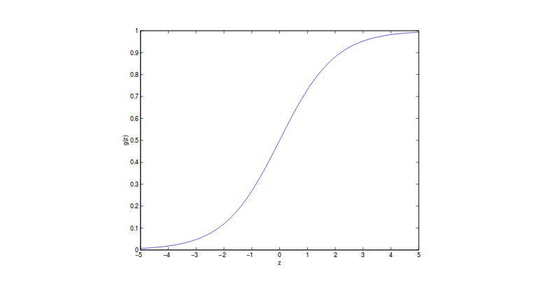
It ranges from 0 to 1 as output. This intuitively explains why we call it regression since it outputs in a continuous space. However, the value indicates the probability of belonging to certain class. So essentially it is a classifier.
let’s look at what it will be when we take derivative of logistic funciton:
\[\begin{align} \frac{d}{dz} g(z) &= \frac{1}{(1+\exp(-z))^2}\big(\exp(-z)\big)\\ &= \frac{1 + \exp(-z) - 1}{(1+\exp(-z))^2} \\ &= \frac{1}{(1+\exp(-z))}\Big(1 - \frac{1}{1+\exp(-z)}\Big)\\ &= g(z)(1-g(z)) \end{align}\]With this prior knowledge, the question is how are we supposed to find $\theta$. So we know least square regression can be derived from maximum likelihood algorithm, which is where we should start from.
We assume:
\[P(y \lvert x;\theta) = (h_{\theta}(x))^y (1 - h_{\theta}(x))^{1-y}\]where y should be either one or zero. Assuming that samples are iid, we have likelihood as:
\[\begin{align} L(\theta) &= \prod_{i=1}^{m} p(y^{(i)}\lvert x^{(i)};\theta)\\ &= \prod_{i=1}^{m} (h_{\theta}(x^{(i)}))^{y^{(i)}} (1 - h_{\theta}(x^{(i)}))^{1-y^{(i)}} \end{align}\]Applying log, we can have:
\[\log L(\theta) = \sum\limits_{i=1}^m y^{(i)}\log h(x^{(i)}) + (1-y^{(i)})\log(1-h(x^{(i)})\]Then, we can use graident descent to optimize the likelihood. In updating, we should have $\theta = \theta + \alpha\triangledown_{\theta}L(\theta)$. Note we have plus sign instead of minus sign since we are finding max not min. To find the derivative,
\[\begin{align} \frac{\partial}{\partial\theta_j}L(\theta) &= \bigg(y\frac{1}{g(\theta^Tx)}-(1-y)\frac{1}{1-g(^Tx)}\bigg)\frac{\partial}{\partial\theta_j}g(\theta^Tx)\\ &= \bigg(y\frac{1}{g(\theta^Tx)}-(1-y)\frac{1}{1-g(^Tx)}\bigg) g(\theta^Tx)* \\ &(1 - g(\theta^Tx))\frac{\partial}{\partial\theta_j}\theta^Tx\\ &= (y - h_{\theta}(x))x_j \end{align}\]From the fisrt line to second line, we use the derivative of logistic function derived above. This gives us the update rule for each dimension on feature vector. Although we have same algorithm as LMS in this case, the hypothesis in this case is different. It is not surprising to have the same equation when we talk about Generalized Linearized Model.
6 Digression: The Perceptron Learning Algortihm
We will talk about this in Learning Theory in more detials. In short, we change our hypothesis function to be:
\[g(\theta^Tx) = \begin{cases} 1 \text{, if } \theta^Tx \geq 0 \\ 0 \text{, otherwise} \\ \end{cases}\]The updating equation remains the same. This is called perceptron learning algorithm.
7 Newton’s Method for Maximizing
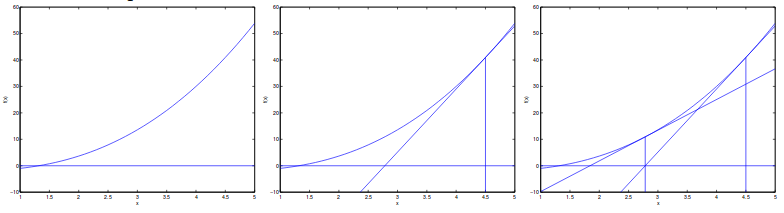
So imagine that we want to find the root of a function f. Newton’s method allows us to do this task in quadratic speed. The idea is to initialize $x_0$ randomly and find the tangent line of $f(x_0)$,dentoed $f^{\prime}(x_0)$. We use the root of $f^{\prime}(x_0)$ as new x. We also define the distance between new x and old x as $\Delta$. An example of this can be shown as:
So we now have:
\[f^{\prime}(x_0) = \frac{f(x_0)}{\Delta} \Rightarrow \Delta = \frac{f(x_0)}{f^{\prime}(x_0)}\]Derived from this idea, we can let $f(x) = L^{\prime}(\theta)$. Going this way, we can find max of objective function faster. For finding min, it is similar.
If $\theta$ is vector-valued, we need to use Hessian in the updating. More details about Hession can be found in the other post. In short, to update, we have:
\[\theta = \theta - H^{-1}\triangledown_{\theta}L(\theta)\]Alhtough it converges in quadratic, each updating is more costly than gradient descent.
8 Generalized Linear Models and Exponential Family
Remeber that we have “coincidence” where the updating of logistic regression and least mean square regression ends up with same form. They are special cases in the big family called GLM. The reason why it is called linear is because every distribution in this family places a linear relationship between varaibles and their weights.
Before going to GML, we fisrt talk about exponential family distributions as the foundation to GLM. We define that a class of distribution is in the exponential family if it can be written in the form:
\[p(y;\eta) = b(y)\exp(\eta^T T(y) - a(\eta))\]where $\eta$ is called natural parameter, $T(y)$ is called sufficient statistic and $a(\eta)$ is called log partition fucntion. Usually, $T(y) = y$ is our case. the term $-a(\eta)$ is the normalizing constant.
T,a and b are fixed parameters with which we can vary $\eta$ to establish different distribution in a class of distributuion. Now, we can show that Bernoulli and Gaussian belong to exponential family.
Bernoulli:
\[\begin{align} p(y;\phi) &= \phi^y(1-\phi)^{1-y}\\ &= \exp(y\log\phi + (1-y)\log(1-\phi))\\ &= \exp\bigg(\bigg(\log\bigg(\frac{\phi}{1-\phi}\bigg)\bigg)y+\log(1-\phi)\bigg) \end{align}\]where:
\[\eta = \log(\phi/(1-\phi))\] \[T(y) = y\] \[a(\eta) = -\log(1-\phi) = \log(1+e^{\eta})\] \[b(y) = 1\]Gaussian:
\[p(y;\mu) = \frac{1}{\sqrt{2\pi}}\exp\bigg(-\frac{1}{2}y^2\bigg)\exp\bigg(\mu y - \frac{1}{2}\mu^2\bigg)\]where $\sigma$ is 1 in this case(we can still do the same thing with varying $\sigma$ and :
\[\eta = \mu\] \[T(y) = y\] \[a(\eta) = \mu^2/2 = \eta^2/2\] \[b(y) = (1/\sqrt{2\pi})\exp(-y^2/2)\]Other exponential distribution: Multinomial, Possion, gamma and exponential, beta and Dirichlet. Since they are all in exponential family, what we can do is to study exponential family in general form and vary $\eta$ to model differently. I will open another section on exponential family.
9 Constructing GLM
As discussed, once we know T,a and b, the family of distribution is already determined. We only need to find $\eta$ to determine the exact distribution.
For example, assume that we want to predict y given x. Before moving on deriving GLM of this regression problem, we make three major assumption about this:
(1) We always assume $y \lvert x;\theta \thicksim \text{ExponentialFamily}(\eta)$.
(2) In general, we want to predict the expected value of T(y) given x. Most likely, we have $T(y) = y$. Formally, we have $h(x) = \mathbb{E}[y\lvert x]$, which is true for both logistic regression and linear regression. Note that in logistic regression, we always have $\mathbb{E}[y\lvert x] = p(y=1\lvert x;\theta)$.
(3) The input and natural parameter are related as:$\eta = \theta^Tx$
9.1 Ordinary Least Squares
In this case, we have $y\thicksim \mathcal{N}(\mu,\sigma^2)$. Previoulsy, we discussed about Gaussian as exponential family. In particular, we have:
\[\begin{align} h_{\theta}(x) &= \mathbb{E}[y\lvert x;\theta]\\ &= \mu\\ &= \eta \\ &=\theta^Tx \end{align}\]where the first equation is from assumption (2); the second is by definition; the third is from early derivation; the last is from assumption (3).
9.2 Logistic Regression
In this setting, we predict either 1 or 0 for class label. Recall that, in Bernoulli, we had $\phi=1/(1+e^{\eta})$. Thus, we can derive the following equation as:
\[\begin{align} h_{\theta}(x) &= \mathbb{E}[y\lvert x;\theta]\\ &= \phi\\ &= 1/(1+e^{-\eta}) \\ &= 1/(1+e^{-\theta^Tx}) \end{align}\]This partially explains why we came up with the form like sigmoid function. Because we assume that y follows from Bernoulli given x, it is natural to have sigmoid function resulted from exponential family. To predict, we think that expected value of $T(y)$ with respect to $\eta$ is a reasonable guess, namely canonical response function or inverse of link function. In general, response function is the function of $\eta$ and gives the relationships between $\eta$ and distribution parameters, while link function produces $\eta$ as a function of distribution parameter. The inversion means to express one in terms of the other, which has nothing to do with mathematical meaning of inversion. From the derivation above, we know that the canonical response function of Bernoulli is logistic function and that of Gaussian is mean function.
9.3 Softmax Regression
In a broader case, we can have multiple classes instead of binary classes above. It is natural to model it as Multinomial distribution, which also belongs to exponential family that can be derived from GLM.
In multinomial, we can define $\phi_1,\phi_2,\dots,\phi_{k-1}$ to be the corresponding probability of $k-1$ classes. We do not need all k classes since last is determined once the previous $k-1$ are set. So we can write $\phi_k = 1-\sum_{i=1}^{k-1}\phi_i$.
We first define $T(y) \in \mathbb{R}^{k-1}$ and :
\[T(1) = \begin{bmatrix} 1\\ 0 \\ \vdots \\ 0 \end{bmatrix}, T(2) = \begin{bmatrix} 0\\ 1 \\ \vdots \\ 0 \end{bmatrix},\dots,T(k) = \begin{bmatrix} 0\\ 0 \\ \vdots \\ 0 \end{bmatrix}\]Note that for $T(k)$, we just have all zeros in the vector since the length of vector is k-1. We let $T(y)_i$ define i-th element in the vector. The definition of indicator is also introduced in course notes, which I am not talking in details here.
Now, we show the steps to derive Multinomial as exponential family:
\[\begin{align} p(y;\phi) &= \phi_1^{\mathbb{1}[y=1]}\phi_2^{\mathbb{1}[y=2]}\dots\phi_k^{\mathbb{1}[y=k]}\\ &= \phi_1^{\mathbb{1}[y=1]}\phi_2^{\mathbb{1}[y=2]}\dots\phi_k^{1 - \sum_{i=1}^{k-1}\mathbb{1}[y=i]}\\ &= \phi_1^{T(y)_1}\phi_2^{T(y)_2}\dots\phi_k^{1 - \sum_{i=1}^{k-1}T(y)_i} \\ &= \exp\Big(T(y)_1\log(\phi_1/\phi_k)+T(y)_2\log(\phi_2/\phi_k) + \dots \\ &+ T(y)_{k-1}\log(\phi_{k-1}/\phi_k)+ \log(\phi_k)\Big) \\ &= b(y)\exp(\eta^TT(y) - a(\eta)) \end{align}\]where
\[\eta = \begin{bmatrix} \log(\phi_1/\phi_k)\\ \log(\phi_2/\phi_k) \\ \vdots \\ \log(\phi_{k-1}/\phi_k) \end{bmatrix}\]and $a(\eta) = -\log(\phi_k)$ and $b(y) = 1$.
This formulates multinomial as exponenital family. We can now have the link function as:
\[\eta_i = \log(\frac{\phi_i}{\phi_k})\]To get the response function, we need to invert the link function:
\[e^{\eta_i} = \frac{\phi_i}{\phi_k}\] \[\phi_k e^{\eta_i} = \phi_i\] \[\phi_k \sum\limits_{i=1}^{k}e^{\eta_i} = \sum\limits_{i=1}^{k} \phi_i\]Then, we have the response function:
\[\phi_i = \frac{e^{\eta_i}}{\sum_{j=1}^{k}e^{\eta_j}}\]This response function is called softmax function.
From the assumption (3) in GLM, we know that $\eta_i = \theta_i^Tx$ for $i=1,2,\dots,k-1$ and $\theta_i \in \mathbb{R}^{n+1}$ is the parameters of our GLM model and $\theta_k$ is just 0 so that $\eta_k = 0$. Now, we have the model based on x:
\[p(y=i\lvert x;\theta) = \phi_i = \frac{e^{\eta_i}}{\sum_{j=1}^{k}e^{\eta_j}} = \frac{e^{\theta_i^T x}}{\sum_{j=1}^{k}e^{\theta_j^Tx}}\]This model is called softmax regression, which is a generalization of logistic regression. Thus, the hypothesis will be:
\[\begin{align} h_{\theta}(x) &= \mathbb{E}[T(y)\lvert x;\theta]\\ &=\begin{bmatrix} \phi_1\\ \phi_2 \\ \vdots \\ \phi_{k-1} \end{bmatrix} \\ &= \begin{bmatrix} \frac{\exp(\theta_1^Tx)}{\sum_{j=1}^k\exp(\theta_j^Tx)}\\ \frac{\exp(\theta_2^Tx)}{\sum_{j=1}^k\exp(\theta_j^Tx)} \\ \vdots \\ \frac{\exp(\theta_{k-1}^Tx)}{\sum_{j=1}^k\exp(\theta_j^Tx)} \end{bmatrix} \end{align}\]Now, we need to fit $\theta$ such that we can max the log likelihood. by definition, we can write it out:
\[\begin{align} L(\theta) &= \sum\limits_{i=1}^m \log(p(y^{(i)}\lvert x^{(i)};\theta)\\ &=\sum\limits_{i=1}^m \log\prod_{l=1}^k\bigg(\frac{\exp(\theta_l^Tx)}{\sum_{j=1}^k\exp(\theta_j^Tx)}\bigg)^{\mathbb{1}\{y^{(i)}=l\}} \end{align}\]We can use gradient descent or Newton’s method to find the max of it.
Note: logistic regression is binary case of softmax regression. Sigmoid function is binary case of softmax function.