EM Algorithm
Introduction
In this section,we will introduce a new learning algorithm for density estimation, namely Expectation-Maximization (EM) algorithm. Before we introduce what EM is, I will first talk about mixture of Gaussian model and build the intuition on that.
Let’s denote ${x^{(1)},\dots,x^{(m)}}$ the training dataset without labels. We assume that each data sample is associated with a class label, say $z^{(i)} \sim Multinomial(\phi)$. So $\phi_j = p(z^{(i)} = j)$. We aslo assume that data samples in each cluster is distributed as Gaussian. That is: $x^{(i)}\lvert z^{(i)}=j\sim\mathcal{N}(\mu_j,\Sigma_j)$. Then, we have joint distribution as $p(x^{(i)},z^{(i)}) = p(x^{(i)}\lvert z^{(i)})p(z^{(i)})$. This looks like k means clustering. This is called mixture of Gaussian. We call $z^{(i)}$ latent variable in this case, meaning it is invisible.
The parameters that are to be optimized are $\phi,\mu,\Sigma$. The likelihood turns out to be:
\[\begin{align} \ell(\phi,\mu,\Sigma) &= \sum\limits_{i=1}^m \log p(x^{(i)};\phi,\mu,\Sigma)\\ &= \sum\limits_{i=1}^m \log \sum\limits_{k=1}^K p(x^{(i)}\lvert z^{(i)}=k;\mu_k,\Sigma_k)p(z^{(i)}=k;\phi) \end{align}\]The standard way is to set its derivatives to zero and solve it with respect to each variable. However, this cannot be solved in a closed form!
Let’s take a look at this equation again. It is hard to solve because we have z variable there. $z^{(i)}$ indicates what class a data sample might belong to. We have to integrate this out, which makes it hard to calculate. If we knew what value z is at the beginning, we can easily calcualte the likelihood as:
\[\ell(\phi,\mu,\Sigma) = \sum\limits_{i=1}^m \log p(x^{(i)}\lvert z^{(i)};\mu_{z^{(i)}},\Sigma_{z^{(i)}}) + \log p(z^{(i)};\phi)\]We set the derivative of this to zero, and then we can update them as:
\[\phi_j = \frac{1}{m}\sum\limits_{i=1}^m \mathbb{1}\{z^{(i)}=j\}\] \[\mu_j = \frac{\sum\limits_{i=1}^m \mathbb{1}\{z^{(i)}=j\} x^{(i)}}{\sum\limits_{i=1}^m \mathbb{1}\{z^{(i)}=j\}}\] \[\Sigma_j = \frac{\sum\limits_{i=1}^m \mathbb{1}\{z^{(i)}=j\} (x^{(i)}-\mu_j)(x^{(i)}-\mu_j)^T}{\sum\limits_{i=1}^m \mathbb{1}\{z^{(i)}=j\}}\]You can calculate them as practice. Note that the frist one is like the one in Gaussian Discriminative Analysis. For second one and third one, these formulas can be useful:
\(\frac{\partial x^TAx}{\partial x} = 2x^TA\) iff A is symmetric and independent of x
\[\frac{\partial \log\lvert X\rvert}{\partial X} = X^{-T}\] \[\frac{\partial a^TX^{-1}b}{\partial X} = -X^{-T}ab^Tx^{-T}\]Again, the proofs of these can be found in Gaussian Discriminative Analysis section.
So we can see that if z is known, we can solve these parameters in one shot. What it essentially means is that if we know the label for each data sample, we can find the proper portion, mean and variance for each cluster easily. This sounds naturally true.
However, when z is unknown, we have to use iterative algorithm to find these parameters. EM comes to play!
If we do not know something, we can take a guess on it. That’s what EM does for us. EM, as name suggested, has two steps, expectation and maximization. In E step, we take a “soft” guess on what value z might be. In M step, it updates the model parameters based on the guess. Remember that if we know z, optimization becomes easier.
1 E Step: for each i,j, $w_j^{(i)} = p(z^{(i)} = j\lvert x^{(i)}; \mu,\Sigma,\phi)$
2 M Step: update parameters:
\(\phi_j = \frac{1}{m}\sum\limits_{i=1}^m w_j^i\)
\(\mu_j = \frac{\sum\limits_{i=1}^m w_j^i x^{(i)}}{\sum\limits_{i=1}^m w_j^i}\)
\(\Sigma_j = \frac{\sum\limits_{i=1}^m w_j^i (x^{(i)}-\mu_j)(x^{(i)}-\mu_j)^T}{\sum\limits_{i=1}^m w_j^i}\)
How do we calculate the E step? In E step, we calculate z by conditioning on current setting of all the parameters, which is the posterior. By using Bayes rule, we have:
\[o(z^{(i)}=j\lvert x^{(i)};\phi,\mu,\Sigma) = \frac{p(x^{(i)}\lvert z^{(i)};\mu,\Sigma)p(z^{(i)};\phi)}{\sum\limits_{k=1}^K p(x^{(i)}\lvert z^{(i)}=k;\mu,\Sigma)p(z^{(i)}=k;\phi)}\]So $w_j^i$ is the soft guess for $z^{(i)}$, indicating that how likely sample i belongs to class j. This is also reflected by the updating euqation where instead of indicator funciton, we have a probablity to sum up. Indicator, on the other hand, is called hard guess. Similar to K means clustering, this algorithm is also susceptible to local optima, so initilizing paramsters several times might be a good idea.
This shows us how EM generally works. I use mixture of Gaussain as an example. Next, I will show why EM works.
The EM algorithm
We have talked about EM algorithm by introducing mixture of Gaussian as an example. Now, we want to analyze EM in mathematical way. How does EM work? Why does it work in general? Does it guarantee to converge?
Jensen’s inequality
Let’s first be armed with the definition of convex function and Jensen’s inequality.
Definition: A function f is a convex function if $f^{\ast\ast}(x)\geq 0$ for $x\in\mathcal{R}$ or its hessian H is positve semi-definite if f is a vector-values function. When both are strictly larger than zero, we call f a strictly convex function.
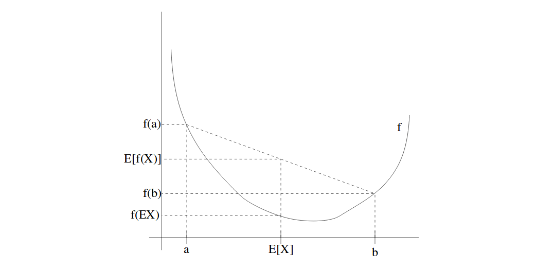
Jensen’s inequality: Let f be a convex function, and let X be a random variable. Then:
\[E[f(X)] \geq f(E[X])\]Moreover, if f is strictly convex, $E[f(X)] = f(E[X])$ is true iff X is constant.
What that means is that with a convex function f, and two points on X-axis with each probability of 0.5 to be selected. We can see that the function value of expected X is less or equal than the expected function value on two points. Such a concept can be visualized in below.
Note This also holds true for concave function since concave funciton is just the reverse of convex function. The inequality is also reversed.
EM Algorithm
With m training samples and a latent variable for each sample, we are trying to maxmimize the likelikhood defined as:
\[\ell(\theta) = \sum\limits_{i=1}^m\log p(x;\theta) = \sum\limits_{i=1}^m\log \sum\limits_z p(x,z;\theta)\]As discussed, it is hard to calculate the derivative of this equation unless z is observed.
EM comes here to solve this issue as shown in last section. Essentially, E-step tries to set a lower bound on loss function, and M-step tries to optimize parameters based on the bound.
Let’s define a distribution on class label for each sample i. We denote $q_i$ be some distribution where $\sum_z q_i(z)=1$. Then, we can extend the likelihood as:
\[\begin{align} \sum\limits_i \log p(x^{(i)};\theta) &= \sum\limits_i\log\sum\limits_{z^i} p(x^{(i)},z^{(i)};\theta)\\ &= \sum\limits_i\log\sum\limits_{z^i} q_i(z^{(i)}) \frac{p(x^{(i)},z^{(i)};\theta)}{q_i(z^{(i)})}\\ &\geq \sum\limits_i\sum\limits_{z^i} q_i(z^{(i)}) \log\frac{p(x^{(i)},z^{(i)};\theta)}{q_i(z^{(i)})} \end{align}\]Last step is from Jensen’s inequality where f is log function. Log function is a concave function and
\[\sum\limits_{z^i} q_i(z^{(i)}) \bigg[\frac{p(x^{(i)},z^{(i)};\theta)}{q_i(z^{(i)})}\bigg] = \mathbb{E}_{z^i\sim q_i(z^{(i)})}\bigg[\frac{p(x^{(i)},z^{(i)};\theta)}{q_i(z^{(i)})}\bigg]\]is the expectation over the random variable defined in the square bracket. Thus, by doing this, we set the lower bound of joint lpg-likelihood.
How do we choose $q_i$? There are many ways to define this distribution as long as it is a simplex. So How do we select from them? When we fix $\theta$, we always to make the bound as tight as possible. When is it the tightest? It is when inequality becomes equality!
How do we make it equal? Remember that for convex/concave function, Jensen’s inequality holds with equality iff the random variable becomes constant. In this case,
\[\frac{p(x^{(i)},z^{(i)};\theta)}{q_i(z^{(i)})} = c\]for some c that does not denpend on $z^i$. We know that if :
\[q_i(z^{(i)}) \propto p(x^{(i)},z^{(i)};\theta)\]then, we can always have a constant as a result. In this case, we can select:
\[\begin{align} q_i(z^{(i)}) &= \frac{p(x^{(i)},z^{(i)};\theta)}{\sum_z p(x^{(i)},z;\theta)}\\ &= \frac{p(x^{(i)},z^{(i)};\theta)}{p(x^{(i)};\theta)}\\ &= p(z^{(i)}\lvert x^{(i)};\theta) \end{align}\]Plugging the RHS in first line will always give a constant for the random variable. The last line just shows that $q_i(z^{(i)})$ is just the posterior of z based on data sample and the parameters.
Let’s put them all together. So we have:
1 E-step: for each i, set:
\[q_i(z^{(i)}) = p(z^{(i)}\lvert x^{(i)};\theta)\]2 M-step: update parameters as :
\[\theta = \arg\max_{\theta} \sum\limits_i\sum\limits_{z^i} q_i(z^{(i)}) \log\frac{p(x^{(i)},z^{(i)};\theta)}{q_i(z^{(i)})}\]We can say that by the end, EM will tell us a point estimate of the best model variables.
The question now is that does this always converge? We want to prove that $\ell(\theta^t)\leq\ell(\theta^{t+1})$. So we have:
\[\begin{align} \ell(\theta^{t+1}) &\geq \sum\limits_i\sum\limits_{z^i} q_i^t(z^{(i)}) \log\frac{p(x^{(i)},z^{(i)};\theta^{t+1})}{q_i^t(z^{(i)})}\\ &\geq \sum\limits_i\sum\limits_{z^i} q_i^t(z^{(i)}) \log\frac{p(x^{(i)},z^{(i)};\theta^{t})}{q_i^t(z^{(i)})}\\ &= \ell(\theta^t) \end{align}\]The first inequality is from Jensen’s inequality which holds for all possible q and $\theta$. The second is because $\theta^{t+1}$ is updated from $\theta^t$ towards the maximization of this likelihood. The last holds because q is chosen in a way that Jensen’s inequality holds with equality.
This shows EM algorithm always converges monotonically. And it will find the optima when updating is small. Note this might not be the global optima.
EM algorithm in general
We have seen that how EM algorithm is derived from mixture of Gaussian and generalized to other cases. In this section, I want to talk about EM algorithm from mathematical point of view in general. That means, instead of deriving from mixture Gaussian, this time we just derive EM algorithm from the beginning without any assumption.
This is an intermediate level of EM concepts. You can skip it if you want.
Setup of EM algorithm
In general, we can abstract traning dataset as X and all the parameters of interets as $\theta$. The model setup can be designed as:
\[X \sim p(X\lvert \theta), \theta \sim p(\theta)\]The goal is to do MAP inference. We want to maximize $\ln p(X,\theta)$ over $\theta$. EM assumes that there is some other variable $\phi$ that we can introduce here so thar marginal distribution is unchanged. That is:
\[p(X, \theta) = \int p(X,\theta,\phi) d\phi\]We want to relate $p(X, \theta)$ and $p(X,\theta,\phi)$ in some way. To move forward, we have:
\[p(X,\theta,\phi) = p(\phi\lvert X,\theta)p(X,\theta)\]We can take log of both sides. Then, we have:
\[\ln p(X,\theta) = \ln p(X,\theta,\phi) - \ln p(\phi\lvert X,\theta)\]We want RHS to be solveable in terms of optimizing $\phi$. If not, there is no point of doing this.
So what have done here is that a new variable $\phi$ is introduced here to help for the MAP inference. The next step is to introduce a distribution of $\phi$ denoted $q(\phi)$ with same support as $\phi$.
We multiply $q(\phi)$ on both sides:
\[q(\phi)\ln p(X,\theta) = q(\phi)\ln p(X,\theta,\phi) - q(\phi)\ln p(\phi\lvert X,\theta)\]Apply integral here:
\[\begin{align} \int q(\phi)\ln p(X,\theta) d\phi &= \int q(\phi)\ln p(X,\theta,\phi) d\phi \\ &- \int q(\phi)\ln p(\phi\lvert X,\theta)d\phi \\ \ln p(X,\theta) \int q(\phi) d\phi&= \int q(\phi)\ln p(X,\theta,\phi) d\phi - \int q(\phi)\ln q(\phi)d\phi \\ &- \int q(\phi)\ln p(\phi\lvert X,\theta)d\phi + \int q(\phi)\ln q(\phi)d\phi \\ \ln p(X,\theta) &= \int q(\phi)\ln p(X,\theta,\phi) d\phi - \int q(\phi)\ln q(\phi)d\phi \\ &- \int q(\phi)\ln p(\phi\lvert X,\theta)d\phi + \int q(\phi)\ln q(\phi)d\phi \end{align}\] \[\ln p(X,\theta) = \int q(\phi)\ln \frac{p(X,\theta,\phi)}{q(\phi)} d\phi + \int q(\phi)\ln \frac{q(\phi)}{p(\phi\lvert X,\theta)}d\phi\]The final equation is called EM master equation. This will help us know what to do and how it works for EM algorithm.
Let’s look at this master equation term by term:
1 $\ln p(X,\theta)$: This is the objective function that we want to optimize.
2 $\mathcal{L}(\theta) = \int q(\phi)\ln \frac{p(X,\theta,\phi)}{q(\phi)} d\phi$ :This is loss function we will discuss later.
3 $KL(q\lvert\rvert p) = \int q(\phi)\ln \frac{q(\phi)}{p(\phi\lvert X,\theta)}$: This is Kullback-Leibler divergence.
KL divergence is a measure of “distance” of two distritbutions on the same support. If two distributions are exactly the same, then KL is zero. Otherwise, the difference is a positive number. That is, KL is a non-negative number.
Let’s look at the master equation:
\[\ln p(X,\theta) = \underbrace{\int q(\phi)\ln \frac{p(X,\theta,\phi)}{q(\phi)} d\phi}_{\mathcal{L}(\theta)} + \underbrace{\int q(\phi)\ln \frac{q(\phi)}{p(\phi\lvert X,\theta)}d\phi}_{KL(q\lvert\rvert p)}\]We can see that changing $q(\phi)$ does not change the final value since LHS does not involve $q(\phi)$, and it only changes how much each part on RHS contributes to the final value. When KL is zero, then loss function is our objective function where $q(\phi) = p(\phi\lvert X,\theta)$. We can use similar form of this to set for q but not exact this one. This is because if we set $q(\phi) = p(\phi\lvert X,\theta)$, then KL diveregnce is always gone for each iteration. There is no point of doing this. It will not help reduce the computational complexity. However, we can take advatange of this form and use q to update $\theta$ and vice versa.
EM algorithm convergence
We want to show that as we update $\theta$, we can have:
\[\ln p(X,\theta_1) \leq \ln p(X,\theta_2) \leq \dots\]At E step:
Set q_t(\phi) = p(\phi\lvert X,\theta_{t-1}) and calculate:
\[\mathcal{L}_t(\theta) = \int q_t(\phi)\ln p(X,\theta,\phi)d\phi - \int q_t(\phi)\ln q_t(\phi) d\phi\]At M step:
We should find:
\[\theta_t = \arg\max_{\theta}\mathcal{L}_t(\theta)\]Note that the second term in loss does not matter for this optimization. We can only focus on the first term.
From this, we can see that it assumes that we can calculate $p(\phi\lvert X,\theta)$ in closed form using Bayes rule. If not, there is no point of moving forward. It also expects that optimization the loss function is easier than optimizing the original objective function.
So in transition from t-1 to t, we have:
\[\begin{align} \ln p(X,\theta_{t-1}) &= \mathcal{L} + KL(q_t\lvert\rvert p(\phi\lvert X,\theta_{t-1})) \\ &= \mathcal{L}_t(\theta_{t-1}) + 0 \\ &\leq \mathcal{L}_t(\theta_t) \\ &\leq \mathcal{L}_t(\theta_{t+1}) + KL(q_t\lvert\rvert p(\phi\lvert X,\theta_t)) \\ &= \ln p(X,\theta_t) \end{align}\]Math: In second line, we know KL is zero which is how we run the algorithm. In third line, it is less than or equal because that is how optimization works. In fourth line, we have KL term there. This time, KL is not zero because $q_t(\phi) = p(\phi\lvert X, \theta_{t-1})$ not $\theta_t$. If they are equal at $\theta_t$, that means it has converged.
By far, I have shown how EM algorithm developes from another perspective, which is more math-dense. This is how EM started from the beginning regardless of any example. I show that they end up with same updating mechanism.
Mixture of Gaussian
Let’s get back to mixture of Gaussian model, a.k.a Gaussian Mixture Model (GMM). I will give a general model for GMM here.
Model: for each $x^i \in \mathbb{R}^d$, given $\pi,\mu,\Sigma$, we have:
\[c^i \sim Discrete(\pi), x^i\lvert c^i \sim \mathcal{N}(\mu_{c^i},\Sigma_{c^i})\]where $c^i$ is the class assignment and we can assign a class index to it. As discussed before, we select the class assignment as our latent variable.
For EM, we always start with:
\[\ln p(x\lvert\pi,\mu,\Sigma) = \sum\limits_c q(c)\ln\frac{p(x,c\lvert \pi,\mu,\Sigma)}{q(c)} + \sum\limits_c q(c)\ln\frac{q(c)}{p(c\lvert x,\pi,\mu,\Sigma)}\]I want to talk about several points here. First, $c=(c^1,c^2,\dots,c^n)$ is a vector and discrete. Thus, we have summations instead of integral. Second, the summation is over all possible values of c, which has $K^n$ possibility. It can easily blow up your memory. It means we need to simplify this, otherwise it has no option of doing this.
EM algorithm says:
E step:
1 Set $q(c) = p(c\lvert x,\pi,\mu,\Sigma)$
2 Calculate $\sum_c q(c)\ln p(x,c\lvert \pi,\mu,\Sigma)$
M step:
We then maximize the above over $\pi,\mu,\Sigma$.
E step:
Use Bayes rule to calculate the conditional posterior:
\[\begin{align} p(c\lvert x,\pi,\mu,\Sigma) &\propto p(x\lvert c,\mu,\Sigma)p(c\lvert\pi) \\ &\propto\prod\limits_{i=1}^n p(x^i\lvert c^i,\mu,\Sigma)p(c^i\lvert\pi) \end{align}\]We need to normalize it with each individual sample:
\[\begin{align} p(c\lvert x,\pi,\mu,\Sigma) &= \prod\limits_{i=1}^n \frac{p(x^i\lvert c^i,\mu,\Sigma)p(c^i\lvert\pi)}{Z_i} \\ &=\prod\limits_{i=1}^n p(c^i\lvert x^i,\pi,\mu,\Sigma) \end{align}\]where
\[\begin{align} p(c^i=k \lvert x^i,\pi,\mu,\Sigma) &= \frac{p(x^i\lvert c^i = k,\mu,\Sigma)p(c^i = k\lvert\pi)}{\sum_{j=1}^K p(x^i\lvert c^i = j,\mu,\Sigma)p(c^i = j\lvert\pi)} \\ &=\frac{\pi_k \mathcal{N}(x^i\lvert\mu_k,\Sigma_k)}{\sum_{j=1}^K \pi_j \mathcal{N}(x^i\lvert\mu_j,\Sigma_j)} \end{align}\]Then, for the loss function:
\[\begin{align} \mathcal{L}(\pi,\mu,\Sigma) &= \sum\limits_{i=1}^n\mathbb{E}_{q(c)}[\ln p(x^i,c^i\lvert \pi,\mu,\Sigma)] + \text{const.} \\ &= \sum\limits_{i=1}^n\mathbb{E}_{q(c^1,\dots,c^n)}[\ln p(x^i,c^i\lvert \pi,\mu,\Sigma)] + \text{const.}\\ &= \sum\limits_{i=1}^n\mathbb{E}_{q(c^i)}[\ln p(x^i,c^i\lvert \pi,\mu,\Sigma)]+ \text{const.} \end{align}\]So the assumption applied here is that each sample with its class assignment is i.i.d. Then the expectation of q(c) with i-th sample is just the expectation of $q(c^i)$ for that sample. By doing this, we do not have to go over all the possibility of c. Instead, we just have Kn terms to deal with. You can see how convenient it is by simply assuming it is iid.
Then, we have:
\[\begin{align} \mathcal{L}(\pi,\mu,\Sigma) &= \sum\limits_{i=1}^n\mathbb{E}_{q(c^i)}[\ln p(x^i,c^i\lvert \pi,\mu,\Sigma)] + \text{const.}\\ &= \sum\limits_{i=1}^n \sum\limits_{j=1}^K q(c^i=j)[\ln p(x^i\lvert c^i=j,\mu,\Sigma) + \ln p(c^i=j\lvert \pi)] \\ &+ \text{const.}\\ &= \sum\limits_{i=1}^n \sum\limits_{j=1}^K \phi_i(j)[\frac{1}{2}\ln\lvert\Sigma_j\rvert -\frac{1}{2}(x^i-\mu_j)^T\Sigma_j(x^i-\mu_j) + \ln\pi_j] \\ &+ \text{const.} \end{align}\]M step:
We want to take the derivative and set to zero.
For $\mu_j$:
\[\triangledown_{\mu_j}\mathcal{L} = -\sum\limits_{i=1}^n \phi_i(j)(\Sigma_j\mu_j - \Sigma_j x^i) = 0\] \[\mu_j = \frac{\sum_{i=1}^n\phi_i(j)x^i}{\sum_{i=1}^n\phi_i(j)}\]For $\Sigma_j$:
\[\triangledown_{\Sigma_j}\mathcal{L} = \sum\limits_{i=1}^n \phi_i(j)(\frac{1}{2}\Sigma_j - \frac{1}{2}(x^i-\mu_j)(x^i-\mu_j)^T)\] \[\Sigma_j = \frac{\sum_{i=1}^n\phi_i(j)(x^i-\mu_j)(x^i-\mu_j)^T}{\sum_{i=1}^n\phi_i(j)}\]For $\pi$:
This step requires the sum over $\pi$ must be 1. We need to apply Lagrange multipliers to do this.
\[\mathcal{L} = \sum\limits_{i=1}^n \sum\limits_{j=1}^K \phi_i(j)\ln\pi_j\]with the constraint $\sum_{j=1}^K \pi_j = 1$. Then, we construct the Lagrangian as:
\[\mathcal{L} = \sum\limits_{i=1}^n \sum\limits_{j=1}^K \phi_i(j)\ln\pi_j +\beta (\sum\limits_{j=1}^K \pi_j -1)\]Take the derivative, we have:
\[\sum\limits_{i=1}^n \frac{\phi_i(j)}{\pi_j} + \beta = 0\]Then, solve it as:
\[\pi_j = \frac{\sum_{i=1}^n \phi_i(j)}{-\beta}\]Using the constraint $\sum_{j=1}^K \pi_j = 1$, we can find:
\[-\beta = \sum\limits_{i=1}^n \sum\limits_{j=1}^K \phi_i(j) = \sum\limits_{i=1}^n 1 = n\]So the update is:
\[\pi_j = \frac{\sum_{i=1}^n \phi_i(j)}{n}\]This concludes our EM algorithm for GMM.
EM for missing data
In this section, I will talk about another example that we can use EM to solve it. It is called missing data problem. In general, we are given the dataset where some of the dataset are observed while others are mising. In this case, we model the missing data with a random variable. This is our latent variable.
Let’s see an example.
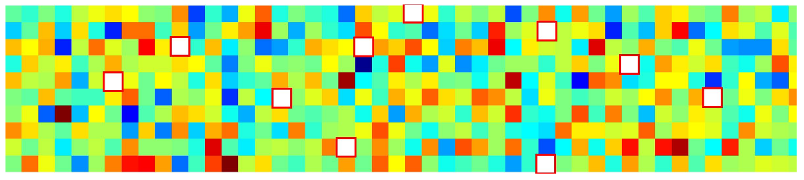
Consider each column as a data sample. We have a couple of missing entries in the data matrix. We can model each column with iid assumption as:
\[x^i\sim \mathcal{N}(\mu,\Sigma)\]We will try to use EM algorithm to fill the missing data intelligently.
As always, we write out the EM master equation with missing data as latent variable. Let’s denote $x_i^o$ as the observed data dimension and $x_i^m$ as the missing data dimension. Then, we have:
\[\sum\limits_{i=1}^m\ln p(x_i^o\lvert \mu,\Sigma) = \sum\limits_{i=1}^m \int q(x_i^m)\ln\frac{p(x_i^o,x_i^m\lvert\mu,\Sigma)}{q(x_i^m)} dx_i^m + \sum\limits_{i=1}^m \int q(x_i^m)\ln\frac{q(x_i^m)}{p(x_i^m\lvert x_i^o,\mu,\Sigma)}\]E step:
1 Set $q(x_i^m) = p(x_i^m\lvert x_i^o,\mu,\Sigma)$ using the most recent $\mu,\Sigma$. We can further think of missing and observed data sample as:
\[x_i = \begin{bmatrix} x_i^o \\ x_i^m \end{bmatrix} \sim \mathcal{N}(\begin{bmatrix} \mu_i^o \\ \mu_i^m \end{bmatrix},\begin{bmatrix} \Sigma_i^{oo} & \Sigma_i^{om} \\ \Sigma_i^{mo} & \Sigma_i^{mm} \end{bmatrix})\]Then, we can show (I will write proof for this if time permitted) that:
\[p(x_i^m\lvert x_i^o,\mu,\Sigma) = \mathcal{N}(\hat{\mu}_i,\hat{\Sigma}_i)\]where
\[\hat{\mu}_i = \mu_i^m + \Sigma_i^{mo}(\Sigma_i^{oo})^{-1}(x_i^o-\mu_i^o)\] \[\hat{\Sigma}_i = \Sigma_i^{mm} - \Sigma_i^{mo}(\Sigma_i^{oo})^{-1}\Sigma_i^{om}\]2 Calculate objective function:
\[\begin{align} \mathbb{E}_{q(x_i^m)}[\ln p(x_i^o,x_i^m\lvert\mu,\Sigma)] &= \mathbb{E}_{q(x_i^m)} [(x_i-\mu)] \\ &=\mathbb{E}_{q(x_i^m)}[(x_i-\mu)^T\Sigma^{-1}(x_i-\mu)] \\ &=\mathbb{E}_{q(x_i^m)}[tr(\Sigma^{-1}(x_i-\mu)(x_i-\mu)^T)] \\ &=tr(\Sigma^{-1}\mathbb{E}_{q(x_i^m)}[(x_i-\mu)(x_i-\mu)^T]) \end{align}\]Recall that $q(x_i^m) =\mathcal{N}(\hat{\mu}_i,\hat{\Sigma}_i). We define:
$\hat{x}_i$: A vector where we replace the missing values in $x_i$ with $\hat{\mu}_i$.
$\hat{V}_i$: A zero matrix plus $\hat{\Sigma}_i$.
M step:
We want to maximize $\sum_{i=1}^m \mathbb{E}_{q(x_i^m)}[\ln p(x_i^o,x_i^m\lvert \mu,\Sigma)]$. The updating can be done:
\[\mu_{new} = \frac{1}{m} \sum\limits_{i=1}^m \hat{x}_i\] \[\Sigma_{new} = \frac{1}{m}\sum\limits_{i=1}^m [(\hat{x}_i - \mu_{new})(\hat{x}_i - \mu_{new}) + \hat{V}_i]\]Then, we return the E step to calculate the new posterior with new $\mu$ and $\Sigma$.
This is just a short example of applying EM in reality.
Summary
EM algorithm is an algorithm which can help reduce the computational load by introducing a new hidden variable. It give us an point estimate of the best possible value for the parameters using iterative optimization. When we say the best, we really mean the best values for maximum likelihood or maximum a posterior. It depends on if we have a model prior in the definition. EM works in both.
The procedure is as follow. First, we select a proper latent variable, which is based on experience. The key is to check the marginal distribution is still correct with the selected latent variable. Second, we caluclate the posterior of this latent variable conditioning on data and current mode parameters. Third, we calculate our objective function using latent variable. This is our E step. At M step, we maximize each model parameter by finding its gradient. We repeat this process until the objective function has converged.